PROCHECK sample plots

Plot 6. Residue properties

Description

The properties plotted are:-

• Graphs a-c: Optional properties

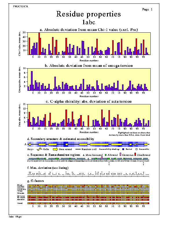
  The first three graphs at the top of the page, can be selected from 14 possibles by the user. The three default graphs, which are plotted when you first run PROCHECK, are the first three of:-

  1. Absolute deviation from mean Chi-1 value (excl. Pro)
  2. Absolute deviation from mean of omega torsion
  3. C-alpha chirality: abs. deviation of zeta torsion
  4. Absolute deviation from mean of H-bond energy
  5. Gamma atom B-value
  6. Average B-value of main-chain atoms
  7. Average B-value of side-chain atoms
  8. G-factor for phi-psi distribution
  9. G-factor for chi1-chi2 distribution
  10. Residue-by-residue G-factor
  11. Approx. accessibility (estimated by Ooi numbers)
  12. Percentage residue main-chain accessibility
  13. Standard deviation of main-chain B-values
  14. Standard deviation of side-chain B-values
  

  For each graph, unusual values (usually those more than 2.0 standard deviations away from the "ideal" mean value) are shown highlighted.

• Graph d: Secondary structure & average estimated accessibility

  The secondary structure plot shows a schematic representation of the Kabsch & Sander (1983) secondary structure assignments. The key just below the picture shows which structure is which. Beta strands are taken to include all residues with a Kabsch & Sander assignment of E, helices corresponds to both H and G assignments, while everything else is taken to be random coil.

  The shading behind the schematic picture gives an approximation to the residue accessibilities. The approximation is a fairly crude one, being based on each residue's Ooi number (Nishikawa & Ooi, 1986). An Ooi number is a count of the number of other Calpha atoms within a radius of, in this case, 14Å of the given residue's own Calpha. Although crude, this does give a good impression of which parts of the structure are buried and which are exposed on the surface. Future versions of PROCHECK will include an accurate calculation of residue accessibility.

• Graph e: Sequence & Ramachandran regions

  The next section shows the sequence of the structure (using the 20 standard one-letter amino-acid codes) and a set of markers that identify the region of the Ramachandran plot in which each residue is located. There are four marker types, one for each of the four different types of region: core (ie most favoured), allowed, generous and disallowed.

• Graph f: Max. deviation

  The small histogram of asterisks and plus-signs shows each residue's maximum deviation from one of the ideal values given on the residue-by-residue listing in the .out file. Refer to the final column of the .out file to see which is the parameter that deviates by the amount shown here.

• Graph g: G-factors

  The shaded squares give a schematic representation of each residue's G-factor values. (Note that the chi-1 G-factors are shown only for those residues that do not have a chi-2, and hence no chi1-chi2 G-factor).

  Regions with many dark squares correspond to regions where the properties are "unusual", as defined by a low (or negative) G-factor. These may correspond to highly mobile or poorly defined regions such as loops, or may need further investigation.

Options

The main options for the plot are:-

• Which 3 of 14 plots to be printed in the 3 main graphs at the top of the page.
• Number of standard deviations for highlighting outliers (default is 2.0).
• The plot can be in colour or black-and-white.

These options can be altered by editing the parameter file, procheck.prm, as described here.

PROCHECK sample plots